

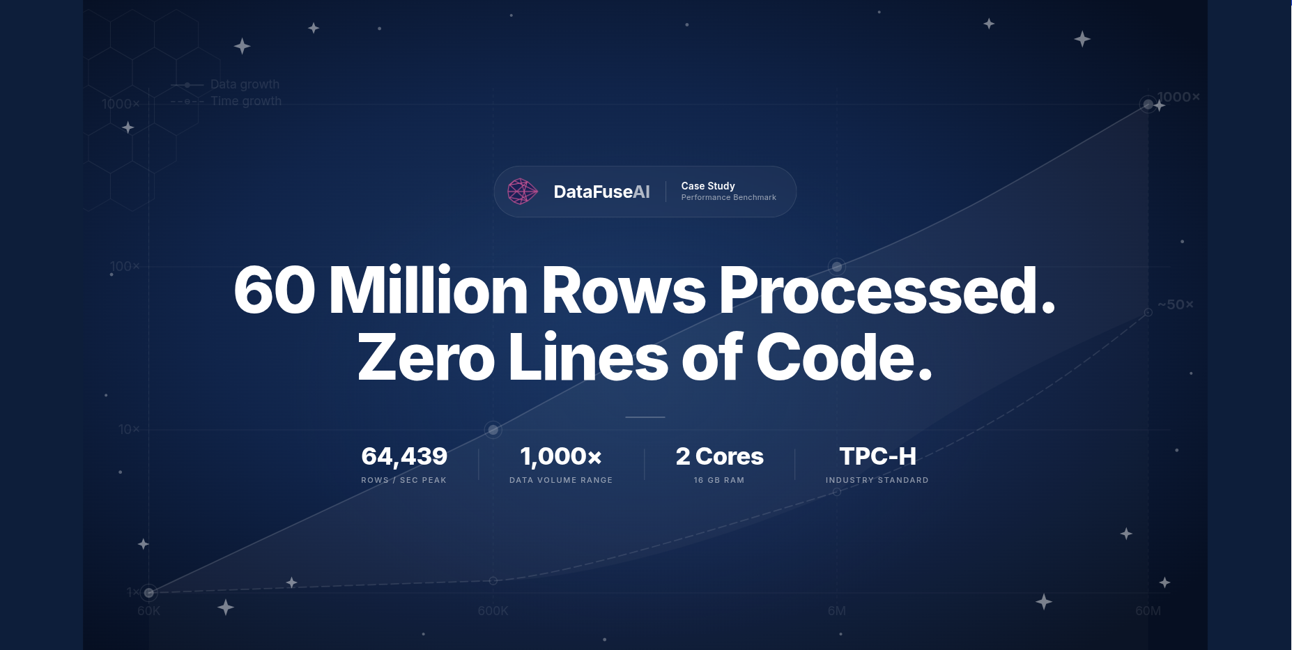
How DataFuseAI Processed 60 Million Rows Without a Single Line of Code
A performance benchmark across 1,000× data volume, four scale factors, and eight real-world ETL pipeline types.
Every Platform Claims It Scales. We Decided to Prove It.
Every data platform says the same thing. In every pitch deck, every landing page, every sales call: “We handle any data volume. We grow with you.”
You’ve heard it before. The real test comes when that promise meets reality. When 60,000 rows become 6 million, and then 60 million. When your joins get heavier, your transformations more complex, and your infrastructure more constrained.
Ask any vendor to publish exactly how long their platform takes to move and transform data at that scale. Ask them to break it down by phase, by pipeline type, by compute environment. Watch how fast the conversation shifts to it depends
and let’s schedule a follow-up.
Scaling a data pipeline is easy in a demo. Proving it is another matter entirely—and proof is what most platforms quietly avoid.
We decided to stop saying it and start showing it.
So we ran the benchmark ourselves: 31 pipeline runs, on a deliberately modest machine, using an industry-standard dataset. We are publishing everything. Every second, every phase, every bottleneck, every constraint. No curation. No convenient rounding. Actual, transparent, reproducible results that show what happens when you push real volume through the system and keep pushing.
This is what happened.
Benchmark Methodology
Dataset: TPC-H (Industry Standard)
The benchmark used TPC-H, the Transaction Processing Performance Council’s decision-support dataset, widely considered the gold standard for testing analytical data workloads. TPC-H isn’t a toy dataset or a synthetic stress test. It simulates what real businesses actually run: aggregations, multi-table joins, filters, and derived calculations at scale. It’s what the industry uses when the goal is honest, comparable measurement.
The focus was on the two heaviest TPC-H tables—lineitem and orders—tested across four volume tiers:
| Scale | Lineitem Rows | Orders Rows | Combined |
|---|---|---|---|
| sf001 | 60,175 | 15,000 | ~75K |
| sf01 | 600,572 | 150,000 | ~750K |
| sf1 | 6,001,215 | 1,500,000 | ~7.5M |
| sf10 | 59,986,052 | 15,000,000 | ~75M |
That’s a 1,000× spread from smallest to largest. The same pipelines, the same platform, across the full range. No shortcuts, no cherry-picked configurations.
Compute: A Realistic, Everyday Setup
This wasn’t run on an enterprise-grade cluster with 64 cores and a terabyte of memory. It ran on the kind of modest setup most smaller teams actually work with day to day:
The choice was deliberate. We wanted to answer a specific question: what happens when you run serious data volume on the kind of hardware that most smaller teams actually have? If DataFuseAI performs at this level on constrained infrastructure, production deployments on properly scaled environments will have real headroom to go further and produce a higher performance.
8 Pipeline Configurations
The benchmark ran across eight distinct pipeline types, covering the transformation patterns most common in real production work. Each one tests a different combination of operations that data teams deal with daily:
| Pipeline | What It Tests |
|---|---|
AGG |
Aggregation on a single large table |
FILTER-AGG |
Filter applied before aggregation |
DERIVED-AGG |
Column derivation followed by aggregation |
ROUTE-AGG |
Multi-sink routing with aggregation |
JOIN-AGG |
Table join, then aggregate |
UNION |
Union across scale factors |
JOIN-SPLIT |
Join into multiple split outputs |
DERIVED |
Full derived column output, no aggregation |
These aren’t theoretical patterns. They’re the building blocks of virtually every ETL workflow in production—from simple single-table rollups to complex multi-source, multi-destination orchestrations.
What the Numbers Show
Sub-Linear Scaling: The Headline Result
The most important finding from this benchmark: data volume grew 1,000×, but total processing time grew just 50×.
| Scale | Avg Rows | Avg Total Time | Avg Throughput |
|---|---|---|---|
| sf001 | 64,461 | 42 sec | 1,571 rows/sec |
| sf01 | 643,429 | 50 sec | 13,420 rows/sec |
| sf1 | 6.4M | 3.1 min | 41,543 rows/sec |
| sf10 | 64.3M | 35.3 min | 37,433 rows/sec |
At 60 million rows, the fastest single pipeline completed in 15.5 minutes. Peak single-run throughput hit 64,439 rows per second—on two cores.
Chart 1
1,000× the Data. 50× the Time.
Two growth curves from the same starting point. The wider the gap, the more efficient the platform. A linearly scaling platform would show both lines tracking together. This one does not.
This sub-linear relationship between data and time is what separates platforms actually designed for scale from platforms that just describe themselves that way. Linear scaling means every 10× increase in data requires a 10× increase in time (and often cost). Sub-linear scaling means the platform gets proportionally more efficient the harder you push it.
How Long Each Scale Actually Takes
Ten times the data. Eight more seconds. That’s what happens from sf001 (60K rows) to sf01 (600K rows). The platform absorbs a full order of magnitude in additional volume with barely a pause. The real climb starts at sf1 (6M rows), and by sf10 (60M rows) total time has grown—but nowhere near proportionally to the data.
Chart 2
The Engine Finds Its Stride Early and Holds It
Average total time at each scale tier. The first two bars are nearly the same height. A 1,000× data increase produced only a 50× time increase.
The Spread Within Each Scale
Average time only tells part of the story. The range between the fastest and slowest pipeline at each scale reveals where the real variation comes from—and where it doesn’t.
Chart 3
Fastest, Average & Slowest Runs at Each Scale
At small scales the three bars sit close together because overhead dominates. At 60M rows the gap opens—driven entirely by how much output each pipeline writes back to PostgreSQL.
At 60 million rows, the fastest run finished in 15.5 minutes. The slowest took 66 minutes. Both ran on the same two cores, through the same platform. The difference comes down to pipeline type and how much output each one writes—not the engine itself. Pipelines that aggregate data down to a small result set finish fast. Pipelines that write millions of rows back to PostgreSQL take longer because the destination is the constraint, not the platform.
Where the Time Goes
Raw totals are useful. But understanding where the time goes tells you something deeper about how the platform is built—and whether it was built well.
Every run was tracked across four phases: Read, Transform, Write, and Overhead (session setup, query planning, orchestration coordination). The breakdown across scale tiers reveals a clear pattern:
| Scale | Read | Transform | Write | Overhead |
|---|---|---|---|---|
| sf001 (60K) | 6.1% | 10.8% | 12.3% | 70.8% |
| sf01 (600K) | 7.0% | 14.5% | 23.1% | 55.4% |
| sf1 (6M) | 6.0% | 31.0% | 44.1% | 18.9% |
| sf10 (60M) | 4.3% | 35.1% | 57.1% | 4.5% |
At small volumes, session setup and query planning naturally dominate. There’s simply not much data to move, so initialization is the largest share of total time. But as volume increases, that overhead compresses dramatically. By 60 million rows, overhead has shrunk to just 4.5% of total time. The engine is spending over 92% of its runtime on actual data work: reading, transforming, and writing.
Chart 4
A Platform That Gets More Productive the Harder You Push It
Each bar adds to 100%. The light section (overhead) shrinks from 70.8% at 60K rows to just 4.5% at 60M rows.
Key Insight: Orchestration overhead grew only 2.4× while data grew 1,000×. The orchestration layer does not bloat. It stays lean and stays out of the way. That’s a signal of how the platform was architected, not just how fast it runs.
The absolute numbers behind that story are just as revealing. Overhead barely moves across the entire 1,000× range. Write time climbs the steepest at scale—and that’s a PostgreSQL insertion constraint, not a platform one.
Chart 5
One Line Barely Moves. One Climbs Steeply. They Are Not the Same Problem.
Growth multiplier per phase. Read grows 26×, Transform 141×, Write 245×, and Overhead (dashed) just 2.4×.
The Bottleneck Tells the Story
At each scale factor, the dominant constraint shifted to a different layer. The progression tells you exactly what kind of system you’re looking at:
| Scale | Dominant Bottleneck |
|---|---|
| sf001 (60K) | Engine initialization (overhead) |
| sf01 (600K) | Engine initialization (overhead) |
| sf1 (6M) | Transformation computation |
| sf10 (60M) | Destination database writes |
At no scale was DataFuseAI itself the limiting factor. As volume grew, the bottleneck moved naturally outward. First to the computational load of joins and aggregations. Then to the ingestion capacity of the PostgreSQL destination. The platform consistently processed its work ahead of what the external systems could absorb.
That is the right dynamic. A well-built pipeline platform should complete its own work faster than the systems it connects to can keep up. The bottleneck should always be somewhere else: in the database, in the network, in the compute layer. Never in the orchestration and transformation engine itself.
The 60 Million Row Runs, Up Close
The sf10 scale was the real test. Nearly 60 million rows pushed through joins, aggregations, filters, derived columns, and route-splits—on a machine with just two cores and 16 GB of memory.
| Pipeline | Input Rows | Total Time | Throughput | Bottleneck |
|---|---|---|---|---|
AGG |
59.99M | 15.5 min | 64,439 r/s | Write |
JOIN-AGG |
74.99M | 21.4 min | 58,400 r/s | Transform |
DERIVED-AGG |
59.99M | 22.5 min | 44,365 r/s | Transform |
FILTER-AGG |
59.99M | 35.2 min | 28,382 r/s | Write |
DERIVED |
59.99M | 36.4 min | 27,435 r/s | Write |
ROUTE-AGG |
59.99M | 49.6 min | 20,149 r/s | Transform |
JOIN-SPLIT |
74.99M | 66.3 min | 18,863 r/s | Write |
The ranking by throughput shows a clear and consistent pattern. Aggregation pipelines—where output row counts are small—finish fastest because the write load is minimal. Write-heavy pipelines that push millions of output rows back into PostgreSQL take longer. The platform is not the variable. Output volume is.
Chart 6
Pipeline Throughput at 60 Million Rows — Fastest to Slowest
Seven pipelines ranked by rows/sec. Top to bottom is low-write to high-write workloads.
The most write-intensive run was JOIN-SPLIT: joining 75 million rows and writing nearly 60 million output rows back to PostgreSQL. It completed in just over an hour on two cores. The volume of data being pushed into the destination database—not the pipeline platform—was the defining constraint.
Our Proof: Samples from the sf10 Runs
We don't show number, we present the proof.Below are direct screenshots taken from DataFuseAI during the sf10 benchmark runs—the same runs that produced the timing and throughput figures reported throughout this article. Each screenshot shows the completed pipeline, its recorded run time, and the status of the execution as logged by the platform.
These are unedited captures. No post-processing, no synthetic timing overlays. What you see is what the platform recorded.
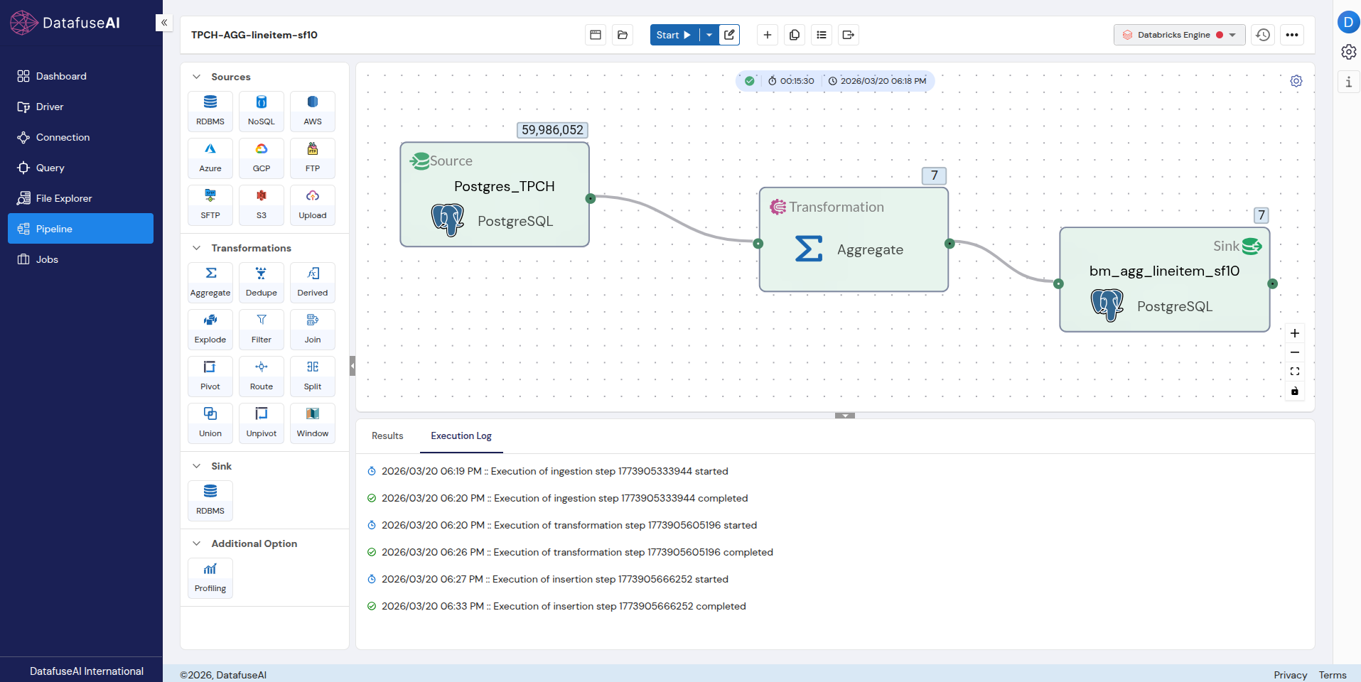
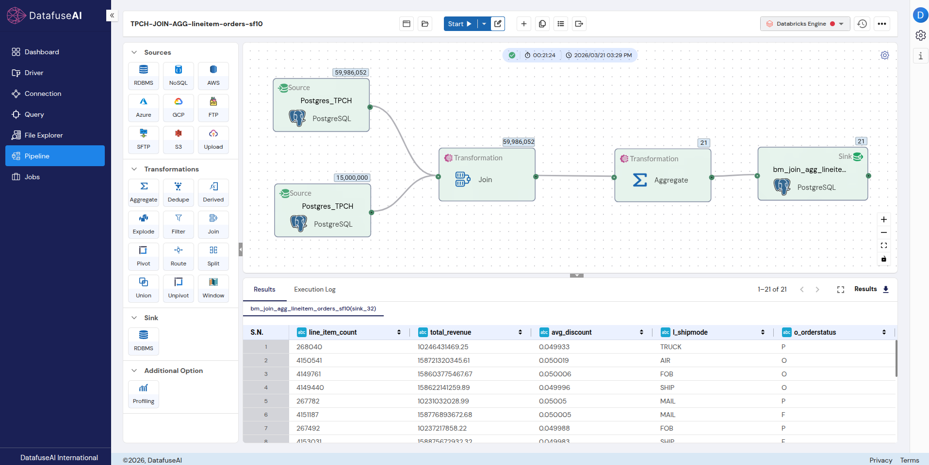
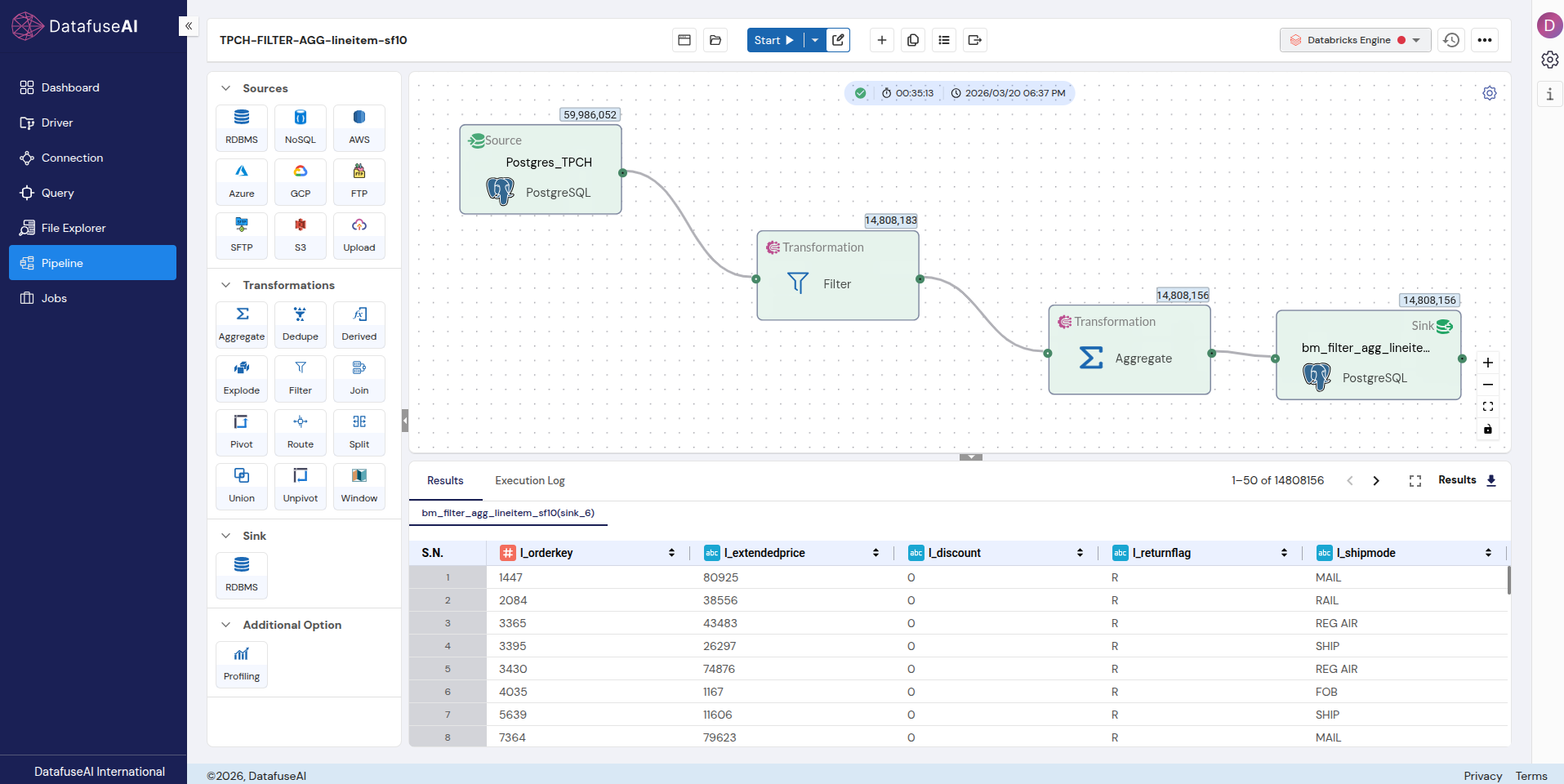
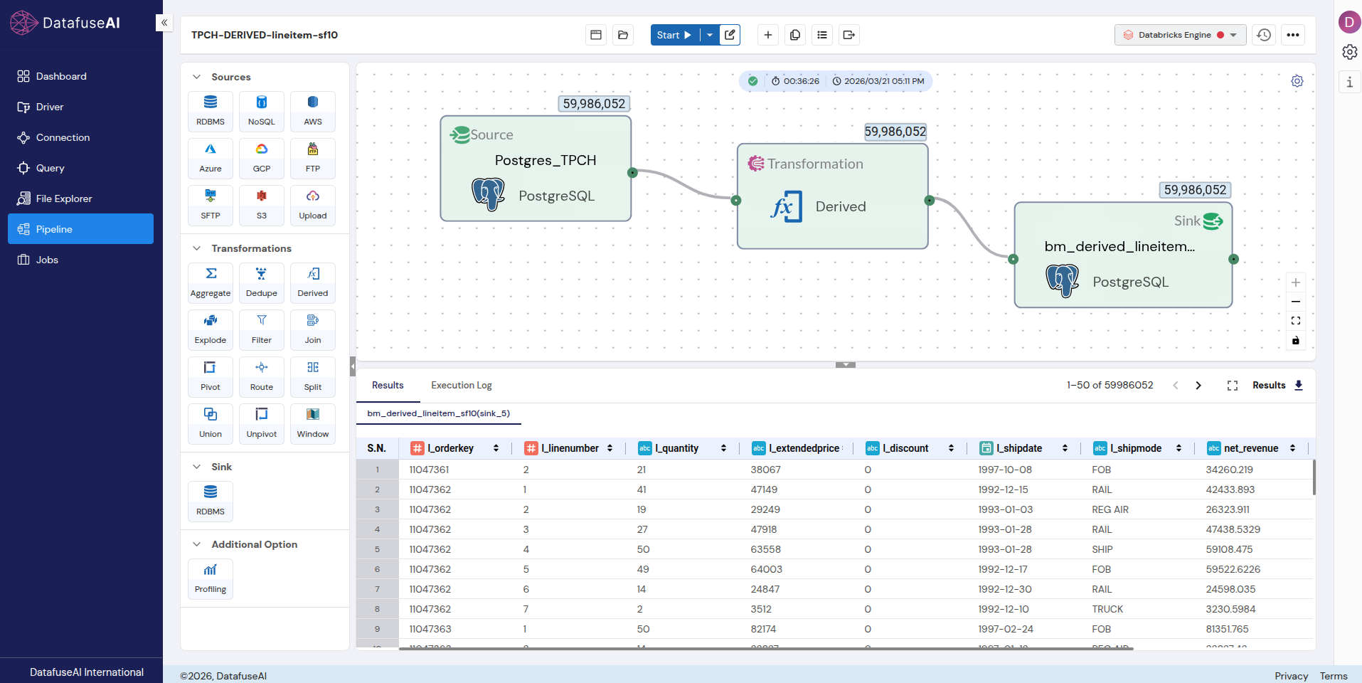
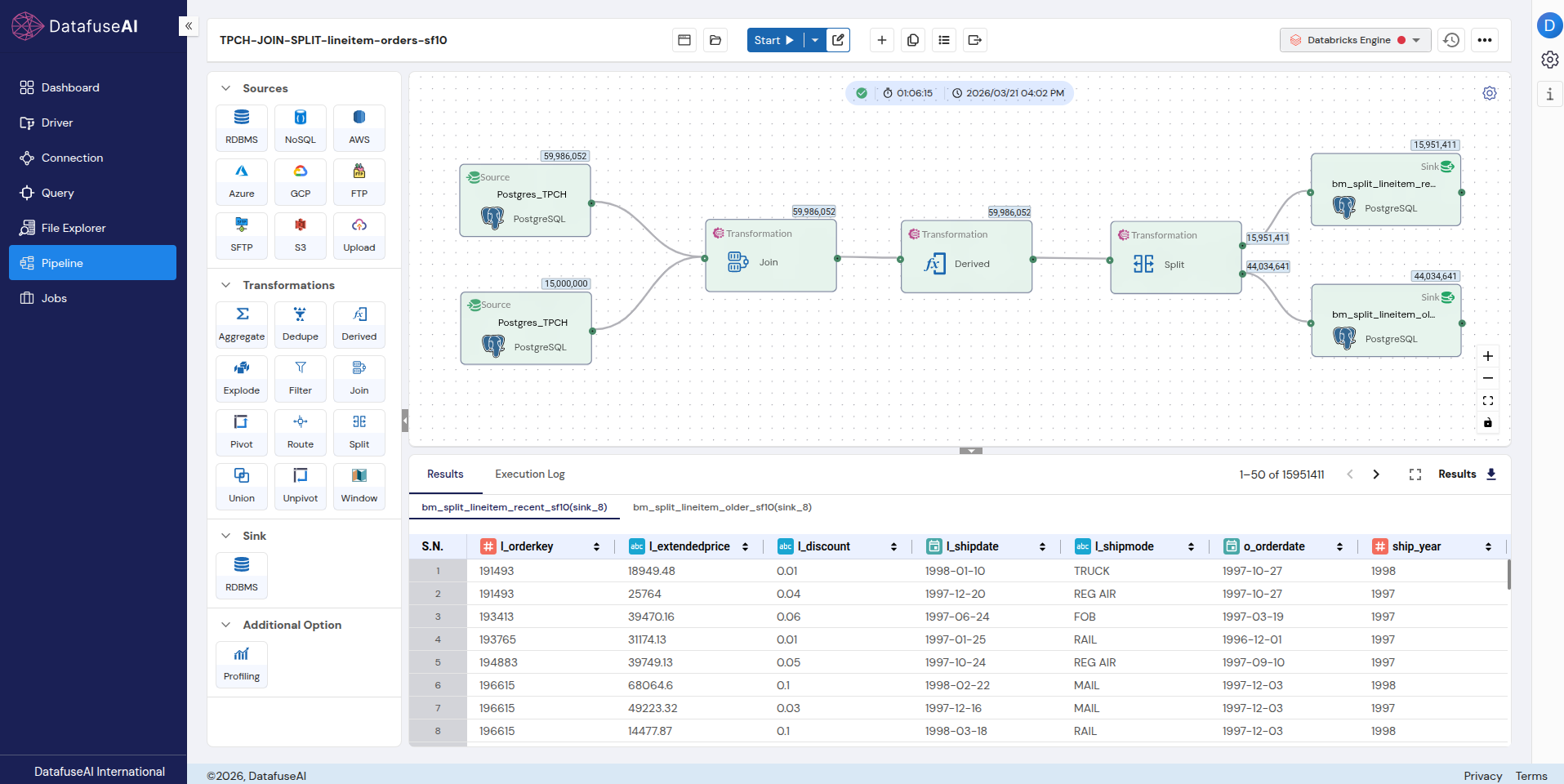
What these screenshots confirm: Every run shown above completed with a Succeeded status. Total run times match the figures reported in the benchmark table. The slowest run shown—JOIN-SPLIT at 66 minutes—processed a combined 74.99 million rows and wrote nearly 60 million output rows back to PostgreSQL, entirely on a two-core machine. These are not test-environment numbers. They are the actual platform, doing actual work, at actual scale.
What This Means in Practice
Volume Handling, Confirmed
DataFuseAI completed complex ETL pipelines at 60 million rows on hardware well within the range of typical team environments. Throughput climbed from 1,571 rows per second at the smallest scale to a peak of 64,439 rows per second at the largest. That’s a 41× improvement, driven by the engine shifting from warm-up overhead into full productive work.
Chart 7
How Throughput Grows as the Engine Shifts from Warm-Up to Full Work
Average throughput vs peak single-run throughput at each scale. By 60M rows the peak reaches 64,439 rows/sec.
Economical Scaling
A 1,000× increase in data volume translated to just a 50× increase in processing time, on a two-core machine. Organizations growing their data operations do not need to proportionally scale their infrastructure to keep pace. The cost per unit of data drops sharply as volume rises—and then holds steady.
No Code Required
Every pipeline in this benchmark—joins, aggregations, derived columns, multi-sink routing—was built using DataFuseAI’s visual drag-and-drop interface. The same no-code environment a business analyst would use for a simple pipeline is the same one that handled 60 million rows of TPC-H data. There is no separate “power mode” or hidden scripting layer required to reach production scale.
Scale, efficiency, and accessibility rarely show up together.
Most platforms force you to trade one for another. You get power but lose simplicity, or you get ease of use but hit a ceiling at real volume. DataFuseAI delivered all three in the same benchmark, on the same hardware, in the same interface.
What Wasn’t Optimized (And What That Means for You)
The benchmark was intentionally run under generalized, untuned conditions to establish an honest baseline:
- All PostgreSQL tables were unindexed, with no partitioning or query optimization applied
- Compute was the smallest practical setup: single node, 2 cores, 16 GB
- Batch sizes and parallelism were not tuned per pipeline or workload
- No PostgreSQL configuration tuning of any kind was applied
In a production deployment, each of these variables would be addressed. Indexed tables, multi-node clusters, tuned sink configurations, optimized batch sizing. Each of these would push performance further—some significantly.
Important: The numbers published here represent a conservative baseline, not a ceiling. They show what the platform does when nothing else is helping. In production, everything else helps.
Summary
31 pipelines. 4 scale factors. 8 pipeline types. A 1,000× range in data volume. Every second tracked and published.
DataFuseAI processed 60 million rows through complex ETL transformations—joins, aggregations, derived columns, multi-sink routing—on a 2-core, 16 GB machine.


 Request a Demo